SeisFlows in Containers
As part of the NSF-funded SCOPED project SeisFlows has been containerized using Docker, which removes the oftentimes troubling task of installing and configuring software. These containers can be used to run SeisFlows on workstations (using Docker) or on high performance computers using Singularity/Apptainer.
Note
The SeisFlows Docker image can be found here: https://github.com/SeisSCOPED/adjtomo
The remainder of this documentation page assumes you are familiar with Docker and containers.
To learn more about Docker and containers, see: https://www.docker.com/resources/what-container/
For instructions to install Docker on your workstation, visit: https://docs.docker.com/get-docker/
Workstation example with Docker
Here we will step through how to run the SeisFlows-SPECFEM2D example using Docker. First we need to get the latest version of the Pyatoa Docker image:
docker pull ghcr.io/seisscoped/adjtomo:latest
Note
These docs were run using Docker image ID c57883926aae (last accessed
Aug. 24, 2022). If you notice that the docs page is out of date with respect
to the latest Docker image, please raise a
SeisFlows GitHub issue.
Their are two methods for running the SeisFlows example using this Docker image, either 1) through a JupyterHub interface, or 2) via the command line. The former provides a graphical user interface that mimics a virtual desktop for easier navigation, while the latter provides a push-button approach.
From JupyterHub
We can run SeisFlows through JupyterHub by opening the container through a port:
docker run -p 8888:8888 \
    --mount type=bind,source=$(pwd),target=/home/scoped/work
    ghcr.io/seisscoped/pyatoa:latest
Warning
If you do not use the --mount command, all progres will be lost
once you close the container. See the
Docker bind mounts
documentation for more information.
To access the JupyterHub instance, open the URL that was output to the display in your favorite web browser. The URL will likely look something like http://127.0.0.1:8888/lab?token=??? where ‘???’ is a unique token
Within the JupyterHub instance, you will be greeted with a graphical user interface (see below). The Pyatoa, PySEP and SeisFlows repositories are navigable in the file system on the left-hand side of the window.
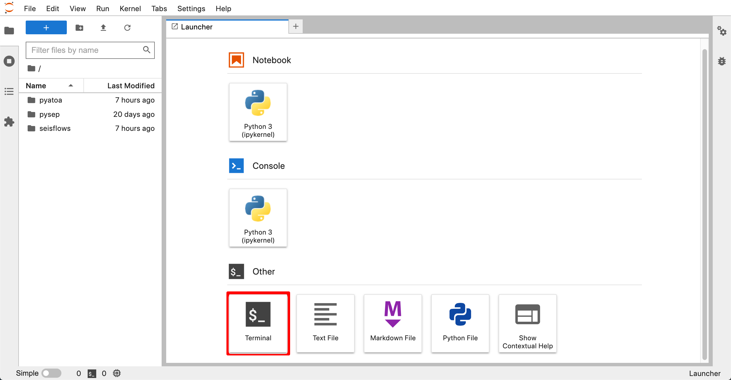
From inside the JupyterHub instance, click the Terminal icon (highlighted red above) to open up a terminal window. Using the terminal we will run our example in an empty directory to avoid muddling up the home directory.
# From inside the JupyterHub terminal
mkdir sf_sem2d_example
cd sf_sem2d_example
seisflows examples run 2
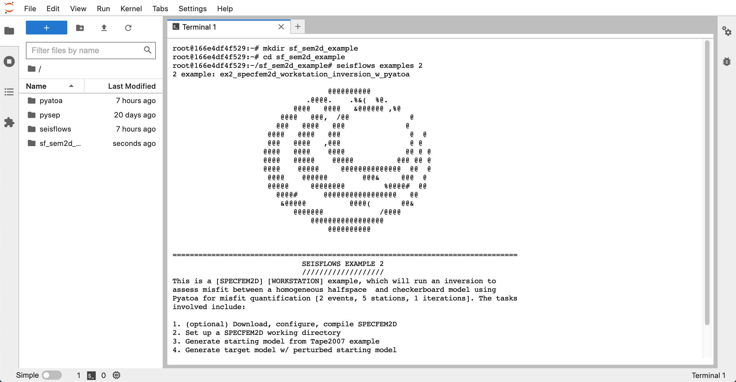
This example will download, configure and compile SPECFEM2D, and then run a SeisFlows-Pyatoa-SPECFEM2D inversion problem. See the SPECFEM2D example docs page for a more thorough explanation of what’s going on under the hood.
A successful inversion
From the command line
Running the container from the command line is much simpler. To print the SeisFlows help message, we simply have to run the following:
docker run ghcr.io/seisscoped/adjtomo:latest seisflows -h
The following code snippet will run a SeisFlows-Pyatoa-Specfem2D example. The extra fluff in the command allows the container to save files to your computer while it runs the example.
WORKDIR=/Users/Chow/Work/scratch  # choose your own directory here
cd ${WORKDIR}
docker run \
    --workdir $(pwd) \
    --mount type=bind,source=$(pwd),target=$(pwd),
    ghcr.io/seisscoped/adjtomo:nightly \
    seisflows examples run 2
In the above example, we set the working directory (-w/–workdir) to the current working directory (on the local filesystem). We also mount the current working directory inside the container (–mount), meaning the container has access to our local filesystem for reading/writing. We then use the Docker image to run a SeisFlows-Pyatoa-Specfem2D example. Outputs of the example will be written into the working directory (WORKDIR).
See the SPECFEM2D example docs page for a more thorough explanation of what’s going on under the hood.
HPC example with Apptainer/Singularity
Note
Section Under Construction
Apptainer/Singularity is a container system for high performance computers (HPC) that allows Users to run container images on HPCs. You might want to use Apptainer if you cannot download software using Conda on your HPC, or you simply do not want to go through the trouble of downloading software on your system.
Relevant Links:
Singularity on Chinook: https://uaf-rcs.gitbook.io/uaf-rcs-hpc-docs/third-party-software/singularity
Singularity at TACC: https://containers-at-tacc.readthedocs.io/en/latest/singularity/01.singularity_basics.html
Singularity on Maui: https://support.nesi.org.nz/hc/en-gb/articles/360001107916-Singularity
Note
This section was written while working on TACC’s Frontera, a SLURM system. Instructions may differ depending on your Systems setup and workload manager. Because Singularity cannot be run on the login nodes at TACC, the following code blocks are run in the idev interactive environment.
To download the required image on your system, we first need to load the
singularity module, and then use a familiar pull command.
module load tacc-singularity  # on TACC Frontera
# module load singularity  # on UAF Chinook
singularity pull seisflows.sif docker://ghcr.io/seisscoped/adjtomo:nightly
We have now downloaded our image as a .sif file. To use the image to run the SeisFlows help message:
singularity run seisflows.sif seisflows -h
To get SeisFlows to use your system’s Singularity (if supported), you just need to append ‘-singularity’ to an existing system subclass in the SeisFlows parameter file. For example, since we are running on Frontera, we set our system to ‘frontera-singularity’.
seisflows setup  # create the 'parameters.yaml' file
seisflows par system frontera-singularity  # set the system
# ... set any other main modules here
seisflows configure  # fill out the parameter file
# ... edit your parameters here and then run SeisFlows
singularity run ghcr.io/seisscoped/adjtomo:nightly seisflows submit